 "
]
},
{
"cell_type": "markdown",
"metadata": {},
"source": [
"### Obtain shapefiles from GRID\n",
"Run GRID normally on the image `s1.tif`. The output shapefiles allow us to replicate the plot coordinates to the next season (image).\n",
"
"
]
},
{
"cell_type": "markdown",
"metadata": {},
"source": [
"### Obtain shapefiles from GRID\n",
"Run GRID normally on the image `s1.tif`. The output shapefiles allow us to replicate the plot coordinates to the next season (image).\n",
" "
]
},
{
"cell_type": "markdown",
"metadata": {},
"source": [
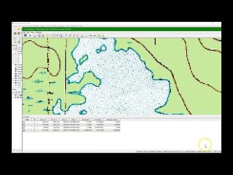
"### Georeference the 2nd image by the 1st image\n",
"**NOTE**: This step can be skipped if the coordinate reference systsm (CRS) of two images matches well.\n",
"\n",
"Before we work with ``s2.tif``, we have to ensure that both ``s1.tif`` and ``s2.tif`` share the same CRS. As the coordinates recorded by GPS may sometimes have error from one image to another, it's necessary to correct the georeference in QGIS. \n",
"
"
]
},
{
"cell_type": "markdown",
"metadata": {},
"source": [
"### Georeference the 2nd image by the 1st image\n",
"**NOTE**: This step can be skipped if the coordinate reference systsm (CRS) of two images matches well.\n",
"\n",
"Before we work with ``s2.tif``, we have to ensure that both ``s1.tif`` and ``s2.tif`` share the same CRS. As the coordinates recorded by GPS may sometimes have error from one image to another, it's necessary to correct the georeference in QGIS. \n",
" "
]
},
{
"cell_type": "markdown",
"metadata": {},
"source": [
"Here's a tutorial on [YouTube](https://www.youtube.com/watch?v=67j_HShwv8Y):\n",
"\n",
"[](https://www.youtube.com/watch?v=67j_HShwv8Y)"
]
},
{
"cell_type": "markdown",
"metadata": {},
"source": [
"### Load shapefiles to replicate CRS\n",
"After we done georeferencing ``s2.tif``, we are ready to replicate the segmetation from `s1.tif` to `s2.tif`. We will load `s2.tif` as the input image this time, and load `s1.shp` as the input shapefile. \n",
"
"
]
},
{
"cell_type": "markdown",
"metadata": {},
"source": [
"Here's a tutorial on [YouTube](https://www.youtube.com/watch?v=67j_HShwv8Y):\n",
"\n",
"[](https://www.youtube.com/watch?v=67j_HShwv8Y)"
]
},
{
"cell_type": "markdown",
"metadata": {},
"source": [
"### Load shapefiles to replicate CRS\n",
"After we done georeferencing ``s2.tif``, we are ready to replicate the segmetation from `s1.tif` to `s2.tif`. We will load `s2.tif` as the input image this time, and load `s1.shp` as the input shapefile. \n",
" "
]
},
{
"cell_type": "markdown",
"metadata": {},
"source": [
"Users are required to crop the area of interest (AOI) and define the pixel of interest (POI). After that, the segmentation will be carried out exactly the same way as one in `s1.tif`.\n",
"
"
]
},
{
"cell_type": "markdown",
"metadata": {},
"source": [
"Users are required to crop the area of interest (AOI) and define the pixel of interest (POI). After that, the segmentation will be carried out exactly the same way as one in `s1.tif`.\n",
" "
]
},
{
"cell_type": "markdown",
"metadata": {},
"source": [
"### Inspect tabular data"
]
},
{
"cell_type": "code",
"execution_count": 1,
"metadata": {},
"outputs": [],
"source": [
"# imports\n",
"import numpy as np\n",
"import pandas as pd\n",
"import os\n",
"import matplotlib.pyplot as plt\n",
"from scipy.stats import pearsonr\n",
"import h5py as h5"
]
},
{
"cell_type": "code",
"execution_count": 3,
"metadata": {},
"outputs": [
{
"data": {
"text/html": [
"
"
]
},
{
"cell_type": "markdown",
"metadata": {},
"source": [
"### Inspect tabular data"
]
},
{
"cell_type": "code",
"execution_count": 1,
"metadata": {},
"outputs": [],
"source": [
"# imports\n",
"import numpy as np\n",
"import pandas as pd\n",
"import os\n",
"import matplotlib.pyplot as plt\n",
"from scipy.stats import pearsonr\n",
"import h5py as h5"
]
},
{
"cell_type": "code",
"execution_count": 3,
"metadata": {},
"outputs": [
{
"data": {
"text/html": [
"| \n", " | id | \n", "canopy_s1 | \n", "ndvi_s1 | \n", "canopy_s2 | \n", "ndvi_s2 | \n", "
|---|---|---|---|---|---|
| 0 | \n", "unnamed_0 | \n", "6139 | \n", "0.079541 | \n", "10756 | \n", "0.057954 | \n", "
| 1 | \n", "unnamed_9 | \n", "5289 | \n", "0.064362 | \n", "11499 | \n", "0.050158 | \n", "
| 2 | \n", "unnamed_18 | \n", "2175 | \n", "0.057072 | \n", "5965 | \n", "0.042233 | \n", "
| 3 | \n", "unnamed_27 | \n", "5958 | \n", "0.060194 | \n", "15209 | \n", "0.040483 | \n", "
| 4 | \n", "unnamed_36 | \n", "3293 | \n", "0.067456 | \n", "8394 | \n", "0.048621 | \n", "
| ... | \n", "... | \n", "... | \n", "... | \n", "... | \n", "... | \n", "
| 265 | \n", "unnamed_233 | \n", "7759 | \n", "0.084310 | \n", "10316 | \n", "0.099573 | \n", "
| 266 | \n", "unnamed_242 | \n", "6455 | \n", "0.050348 | \n", "9391 | \n", "0.068676 | \n", "
| 267 | \n", "unnamed_251 | \n", "4714 | \n", "0.043048 | \n", "10661 | \n", "0.032655 | \n", "
| 268 | \n", "unnamed_260 | \n", "4696 | \n", "0.045965 | \n", "9780 | \n", "0.044229 | \n", "
| 269 | \n", "unnamed_269 | \n", "6703 | \n", "0.079980 | \n", "11354 | \n", "0.061780 | \n", "
270 rows × 5 columns
\n", "| \n", " | id | \n", "canopy_s1 | \n", "ndvi_s1 | \n", "canopy_s2 | \n", "ndvi_s2 | \n", "growth_rate | \n", "isElite | \n", "
|---|---|---|---|---|---|---|---|
| 6 | \n", "unnamed_54 | \n", "2044 | \n", "0.064161 | \n", "6793 | \n", "0.044786 | \n", "2.323386 | \n", "True | \n", "
| 63 | \n", "unnamed_29 | \n", "2274 | \n", "0.116536 | \n", "6812 | \n", "0.094472 | \n", "1.995602 | \n", "True | \n", "
| 105 | \n", "unnamed_138 | \n", "2498 | \n", "0.104650 | \n", "7121 | \n", "0.113467 | \n", "1.850681 | \n", "True | \n", "
| 253 | \n", "unnamed_125 | \n", "2988 | \n", "0.070304 | \n", "8435 | \n", "0.069946 | \n", "1.822959 | \n", "True | \n", "
| 256 | \n", "unnamed_152 | \n", "3094 | \n", "0.078514 | \n", "8665 | \n", "0.060872 | \n", "1.800582 | \n", "True | \n", "
| ... | \n", "... | \n", "... | \n", "... | \n", "... | \n", "... | \n", "... | \n", "... | \n", "
| 170 | \n", "unnamed_185 | \n", "7543 | \n", "0.124144 | \n", "9593 | \n", "0.149356 | \n", "0.271775 | \n", "False | \n", "
| 87 | \n", "unnamed_245 | \n", "7795 | \n", "0.093975 | \n", "9883 | \n", "0.123432 | \n", "0.267864 | \n", "False | \n", "
| 26 | \n", "unnamed_234 | \n", "8109 | \n", "0.087209 | \n", "10260 | \n", "0.107430 | \n", "0.265261 | \n", "False | \n", "
| 172 | \n", "unnamed_203 | \n", "7375 | \n", "0.113576 | \n", "9316 | \n", "0.146696 | \n", "0.263186 | \n", "False | \n", "
| 18 | \n", "unnamed_162 | \n", "8168 | \n", "0.103522 | \n", "9540 | \n", "0.136832 | \n", "0.167973 | \n", "False | \n", "
270 rows × 7 columns
\n", "