Customize Vegetation Indices

Objectives

Derive a index that can better associate with the canopy area of alfalfa than NDVI does. The input image used in this tutorial is an orthoimage with 6 spectral channels. We will demonstrate how to utilize the output files to perform a simple feature selection.

Inspect output files

[1]:

# imports
import os
import numpy as np
import pandas as pd
import matplotlib.pyplot as plt
import matplotlib.image as mpimg
from scipy.stats import pearsonr

[2]:

# inspect the output files
os.listdir()

[2]:

['GRID_bin.png',
 'GRID_seg_border.png',
 'GRID.shx',
 '.DS_Store',
 'GRID.shp',
 'GRID_data.csv',
 'GRID.dbf',
 'GRID_image.npy',
 'GRID_seg_ID.png',
 '.ipynb_checkpoints',
 'GRID_kmeans.png',
 'GRID_raw.png']

[3]:

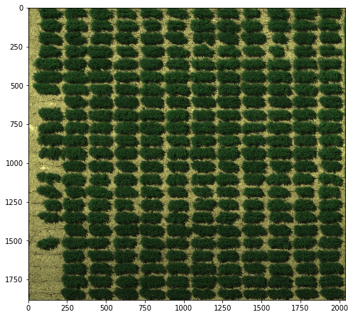
# inspect the input image
img = mpimg.imread('GRID_raw.png')
plt.figure(figsize=(8, 8))
plt.imshow(img)

[3]:

<matplotlib.image.AxesImage at 0x7f94b1002e90>

[4]:

# inspect the tabular output
dt = pd.read_csv("GRID_data.csv"); dt

[4]:

	var	row	col	area_all	area_veg	NDVI	NDVI_std	GNDVI	GNDVI_std	CNDVI	...	ch_2	ch_2_std	ch_3	ch_3_std	ch_4	ch_4_std	ch_5	ch_5_std	ch_6	ch_6_std
0	unnamed_0	1	1	14910	6205	0.680722	0.101848	0.481553	0.086146	0.955003	...	59.423529	15.689919	26.239484	8.893769	167.117808	21.852656	69.889927	10.829972	30.540088	24.633806
1	unnamed_23	1	2	10251	6074	0.676454	0.094532	0.475063	0.077119	0.942506	...	59.718966	14.534593	26.431841	8.389850	165.603721	20.710229	69.595324	9.956617	26.050244	23.631348
2	unnamed_46	1	3	12996	8037	0.679914	0.089733	0.474278	0.074406	0.944246	...	60.750404	14.811752	26.750280	8.541490	167.954585	21.471309	69.989051	10.539928	31.216141	24.766432
3	unnamed_69	1	4	11100	5435	0.643977	0.114235	0.442635	0.088716	0.879109	...	65.185097	15.769556	28.936155	9.405345	166.668813	21.403908	68.871757	10.314017	20.444095	21.586253
4	unnamed_92	1	5	12506	5645	0.659209	0.118899	0.460301	0.092747	0.913120	...	62.443933	16.140226	27.421612	9.592832	166.453853	19.131734	69.195748	9.295681	17.890222	21.159997
...	...	...	...	...	...	...	...	...	...	...	...	...	...	...	...	...	...	...	...	...	...
271	unnamed_183	23	8	13851	6455	0.743537	0.114225	0.598427	0.093205	1.154553	...	44.106274	12.926948	20.407901	8.120920	173.637180	21.825689	72.545778	11.594452	38.396902	19.955167
272	unnamed_206	23	9	12877	6293	0.735538	0.113924	0.594051	0.090958	1.140933	...	44.571746	13.482742	21.143334	8.533524	172.578738	20.879160	72.617670	11.297813	34.843954	19.919131
273	unnamed_229	23	10	12880	7028	0.751853	0.099948	0.605144	0.079713	1.168800	...	43.526323	11.750768	20.231929	7.710727	175.287137	22.499670	74.050370	12.060664	40.409932	21.961529
274	unnamed_252	23	11	13122	6433	0.734485	0.123072	0.590896	0.098009	1.137487	...	45.554018	14.221262	21.560547	9.116043	174.559304	22.556524	73.487331	12.153618	44.907508	16.025357
275	unnamed_275	23	12	15252	7576	0.740249	0.106438	0.593371	0.087980	1.144174	...	45.191526	12.338402	21.199842	8.073755	175.554250	23.091342	74.060058	12.693901	43.955649	18.627713

276 rows × 29 columns

[5]:

# subset columns of canopy area, NDVI, and spectral signals
dt_idx = dt[["area_veg", "NDVI"] + ["ch_%d" % i for i in range(1, 7)]].dropna(); dt_idx

[5]:

	area_veg	NDVI	ch_1	ch_2	ch_3	ch_4	ch_5	ch_6
0	6205	0.680722	32.572442	59.423529	26.239484	167.117808	69.889927	30.540088
1	6074	0.676454	32.683240	59.718966	26.431841	165.603721	69.595324	26.050244
2	8037	0.679914	32.748165	60.750404	26.750280	167.954585	69.989051	31.216141
3	5435	0.643977	36.915731	65.185097	28.936155	166.668813	68.871757	20.444095
4	5645	0.659209	35.175554	62.443933	27.421612	166.453853	69.195748	17.890222
...	...	...	...	...	...	...	...	...
271	6455	0.743537	26.120372	44.106274	20.407901	173.637180	72.545778	38.396902
272	6293	0.735538	27.076593	44.571746	21.143334	172.578738	72.617670	34.843954
273	7028	0.751853	25.338788	43.526323	20.231929	175.287137	74.050370	40.409932
274	6433	0.734485	27.561324	45.554018	21.560547	174.559304	73.487331	44.907508
275	7576	0.740249	26.680042	45.191526	21.199842	175.554250	74.060058	43.955649

270 rows × 8 columns

Design index formulas

[6]:

# make a dictionary of formulas
# where x0 and x1 stand for channel signals from two different (same) columns
ls_formula = {"(x0 - x1) / (x0 + x1)": lambda x0, x1: (x0 - x1) / (x0 + x1),
              "x0 / x1":               lambda x0, x1: x0 / x1,
              "(x0 ^ 2) + (x1 ^ 2)":   lambda x0, x1: (x0 ** 2) + (x1 ** 2)}

Compute correlations

We can compute Pearson’s correlation coefficients between the canopy areas (i.e., the column of “area_veg”) and derived indices

[15]:

# instantiate pandas dataframe
dt_results = pd.DataFrame(columns=["x0", "x1", "formula", "r2"])

# define the loop
cols_ignored = 2  # we won't loop over the first 2 columns, which are canopy and NDVI
p = 6  # number of channels we'd like to loop over

# pairwise iterate through 6 spectral bands
for i in range(p):
    for j in range(p):
        # get band signals and store them in x0 and x1
        x0 = dt_idx.iloc[:, cols_ignored + i]
        x1 = dt_idx.iloc[:, cols_ignored + j]

        # compute 3 indices from x0 and x1
        ls_idx = [list(ls_formula.values())[i](x0, x1) for i in range(3)]

        # store results into a temporary dataframe
        dt_temp = pd.DataFrame({
            "x0":      i,
            "x1":      j,
            "formula": list(ls_formula.keys()),
            "r":       [pearsonr(dt_idx["area_veg"], ls_idx[i])[0]
                        for i in range(3)],
            "r2":      [pearsonr(dt_idx["area_veg"], ls_idx[i])[0] ** 2
                        for i in range(3)]
        })

        # append our result dataframe
        dt_results = dt_results.append(dt_temp)

[8]:

# handle results from zero division error
dt_results.loc[dt_results.r2.isna(), ["r2", "r"]] = 0
dt_results

[8]:

	x0	x1	formula	r2	r
0	0	0	(x0 - x1) / (x0 + x1)	0.000000	0.000000
1	0	0	x0 / x1	0.000000	0.000000
2	0	0	(x0 ^ 2) + (x1 ^ 2)	0.230163	-0.479753
0	0	1	(x0 - x1) / (x0 + x1)	0.124206	-0.352429
1	0	1	x0 / x1	0.134024	-0.366092
...	...	...	...	...	...
1	5	4	x0 / x1	0.010826	0.104048
2	5	4	(x0 ^ 2) + (x1 ^ 2)	0.050595	0.224933
0	5	5	(x0 - x1) / (x0 + x1)	0.000000	0.000000
1	5	5	x0 / x1	0.000000	0.000000
2	5	5	(x0 ^ 2) + (x1 ^ 2)	0.003587	0.059888

108 rows × 5 columns

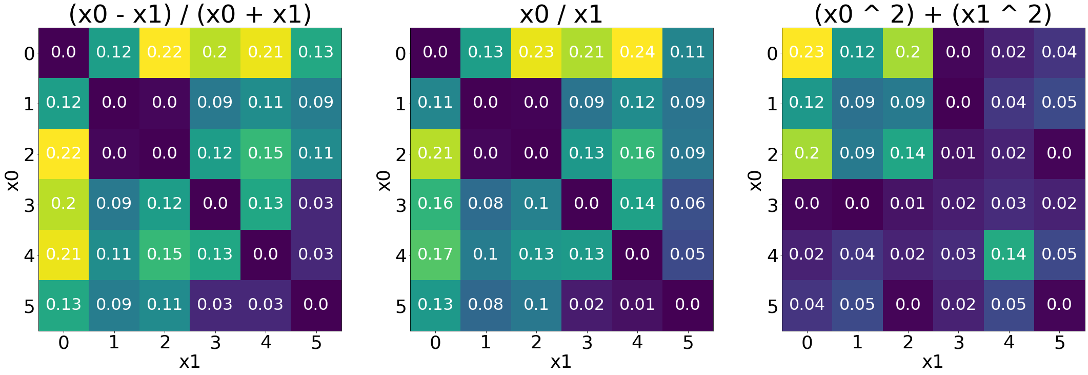
Heatmaps of correlations

This visualization can show how derived indices associate with canopy areas

[9]:

# define font size
size_title = 48
size_label = 32
size_tick  = 36

# generate 3 heatmaps for each formula
fig, axes = plt.subplots(1, 3, figsize=(30, 10), constrained_layout=True)
for i in range(3):
    # get r2 values by each formula
    formula = list(ls_formula.keys())[i]
    ls_r2 = dt_results.loc[dt_results.formula == formula, "r2"]

    # reshape the list to a 2D matrix
    M = np.array(ls_r2).reshape((p, p))

    # plot interface
    axes[i].set_title(list(ls_formula.keys())[i], fontsize=size_title)
    axes[i].set_xlabel("x1", fontsize=size_tick)
    axes[i].set_ylabel("x0", fontsize=size_tick)
    for x0 in range(p):
        for x1 in range(p):
            text = axes[i].text(x0, x1, round(M[x1, x0], 2),
                                ha="center", va="center",
                                color="w", fontsize=size_label)
    plt.sca(axes[i])
    plt.xticks(ticks=np.arange(p), fontsize=size_tick)
    plt.yticks(ticks=np.arange(p), fontsize=size_tick)

    # show heatmap
    axes[i].imshow(M)

../_images/ch4_adv_custom_index_15_0.png

Tabular Results of selected indices

Also we can use in a dataframe to inspect which indices perform better than NDVI

[10]:

# compute correlation between NDVI and canopy area
r2_ndvi = pearsonr(dt_idx["area_veg"], dt_idx["NDVI"])[0] ** 2
r2_ndvi

[10]:

0.1975636107759065

[11]:

# extract rows containing better indices
dt_results.loc[dt_results.r2 > r2_ndvi].sort_values(by="r2", ascending=False)

[11]:

	x0	x1	formula	r2	r
1	0	4	x0 / x1	0.238634	-0.488502
1	0	2	x0 / x1	0.230562	-0.480169
2	0	0	(x0 ^ 2) + (x1 ^ 2)	0.230163	-0.479753
0	0	2	(x0 - x1) / (x0 + x1)	0.220862	-0.469959
0	2	0	(x0 - x1) / (x0 + x1)	0.220862	0.469959
0	0	4	(x0 - x1) / (x0 + x1)	0.214008	-0.462610
0	4	0	(x0 - x1) / (x0 + x1)	0.214008	0.462610
1	2	0	x0 / x1	0.213051	0.461574
1	0	3	x0 / x1	0.209906	-0.458155
2	0	2	(x0 ^ 2) + (x1 ^ 2)	0.199044	-0.446143
2	2	0	(x0 ^ 2) + (x1 ^ 2)	0.199044	-0.446143
0	0	3	(x0 - x1) / (x0 + x1)	0.198422	-0.445445
0	3	0	(x0 - x1) / (x0 + x1)	0.198422	0.445445

Validate the index

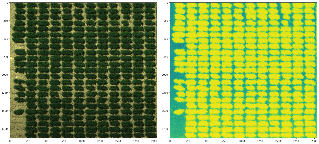
Based on the results shown above, now we know that by dividing the 1st channel by the 5th channel can derive the best canopy-tracking index. we can validate this result by visualize the index as an image.

[13]:

# load image
img = np.load("GRID_image.npy")
img_idx = img[:, :, 0] / (img[:, :, 4] + 1e-9) # adding 1e-9 to avoid zero division error

# as we see the negative correlation,
# we have to treat the largest values as the smallest ones,
# and turn the smallest values to the largest values. (I call it "flip")
img_idx_flip = abs(img_idx - img_idx.max())

# and we can compare the result with the RGB image
fig, axes = plt.subplots(1, 2, figsize=(18, 8), constrained_layout=True)
axes[0].imshow(img[:, :, :3])
axes[1].imshow(img_idx_flip)

[13]:

<matplotlib.image.AxesImage at 0x7f94d05a9c10>

../_images/ch4_adv_custom_index_20_1.png